Linear Shallow Water No Normal Flow Tutorial#
This tutorial will walk you through using an example program that uses the LinearShallowWater2D class to run a simulation with the linear shallow water equations in 2-D. This example is configured using the built in structured mesh generator with no normal flow boundary conditions on all domain boundaries.
Problem Statement#
Equations solved#
In this model, we are solving the linear shallow water equations in 2-D, given by
The variables are defined as follows:
- \(f\) is the background vorticity (set to zero hereafter)
- \(\vec{u} = u \hat{x} + v \hat{y}\) is the barotropic velocity
- \(g\) is the acceleration of gravity
- \(H\) is a uniform resting fluid depth
- \(\eta\) is the deviation of the fluid free surface relative to the resting fluid
In this model, the \(x\) and \(y\) directions are similar to longitude and lattitude, respectively.
Model Domain#
The physical domain is defined by \(\vec{x} \in [0, 1]\times[0,1]\). We use the StructuredMesh routine to create a domain with 20 × 20 elements that are dimensioned 0.05 × 0.05 . Model boundaries are all tagged with the SELF_BC_NO_NORMAL_FLOW flag to implement no normal flow boundary conditions.
Within each element, all variables are approximated by a Lagrange interpolating polynomial of degree 7. The interpolation knots are the Legendre-Gauss points.
Initial and Boundary Conditions#
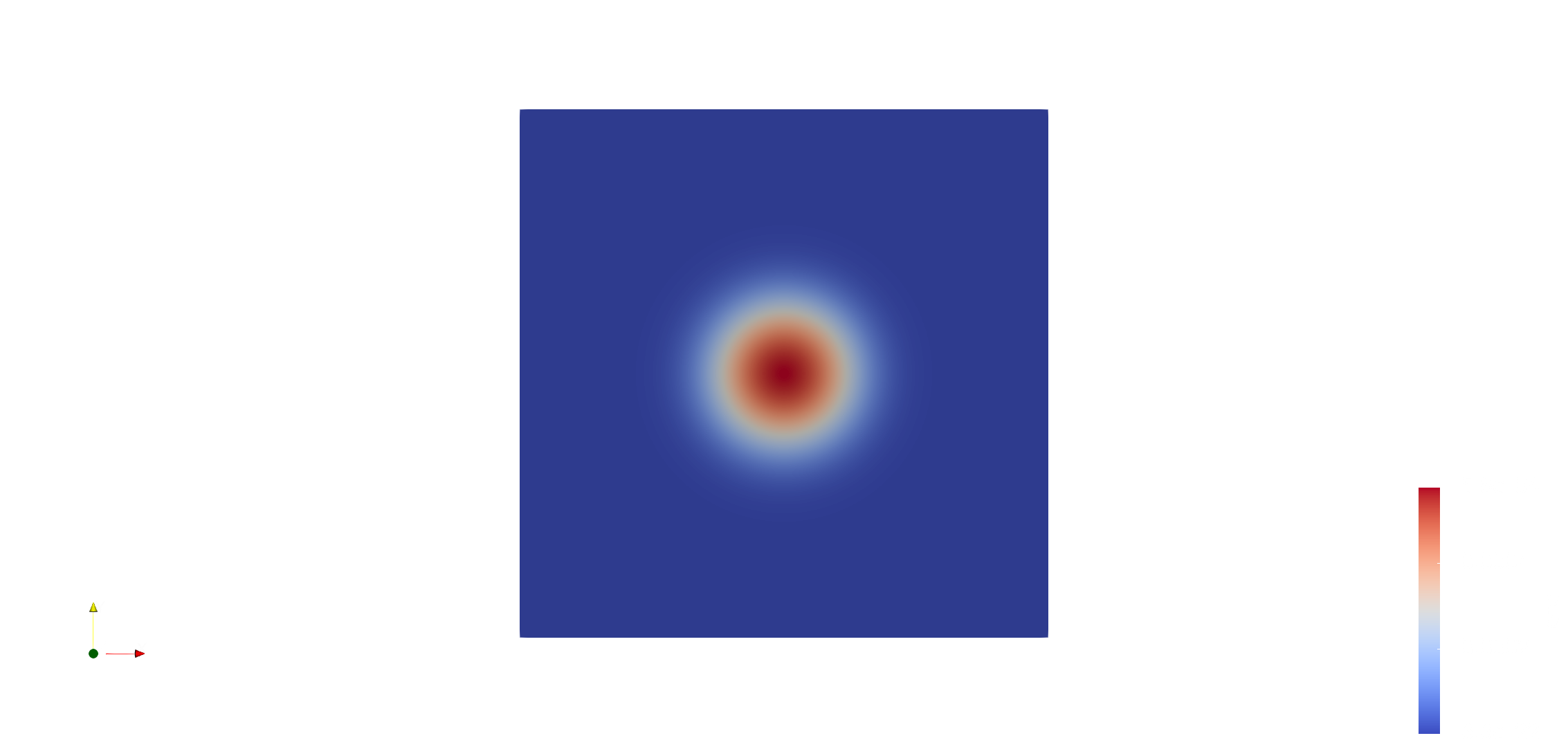
The initial conditions are defined by setting \(x\) and \(y\) velocities equal to zero and the free surface height to a Gaussian centered at \((0.5,0.5)\) with a half-width of \(\approx\) 83mm and a height of 1mm.
Acceleration due to gravity and uniform resting fluid depth are kept constant with \(G = 1.0\) and \(H = 1.0\).
All boundaries are set to no normal flow, i.e., reflecting wave boundary conditions. These are derived using the following assumptions:
- The reflected wave is equal to the incident wave from the fluid interior: $$ \begin{pmatrix} u_L \ v_L \ \eta_L \end{pmatrix} = \begin{pmatrix} u_R \ v_R \ \eta_R \end{pmatrix} $$
- The boundary condition pressure matches the fluid interior pressure.
- The boundary condition tangential velocity matches the fluid interior tangential velocity: $$ -u_R \eta_y + v_R \eta_x = -u_L\eta_y + v_L \eta_x $$
(Subscript \(L\) denotes interior variable and subscript \(R\) denotes exterior variable.)
Together, these conditions imply:
The model is integrated forward in time using \(3^{rd}\) order Runge-Kutta with a time step of \(\Delta t = 0.5 s\).
 Free surface height (
eta) at time t=0.
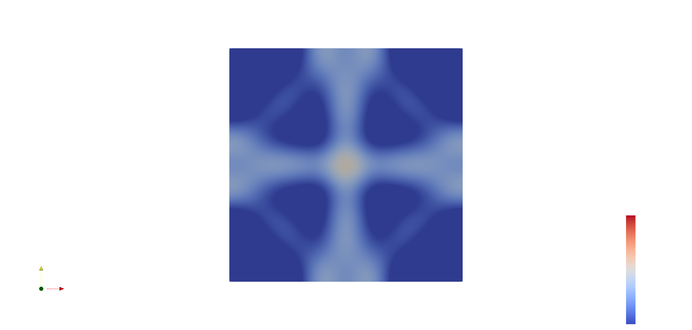
 Free surface height (
eta) at time t=1.
How we implement this#
You can find the example file for this demo in the examples/linear_shallow_water2d_nonormalflow.f90 file. This file uses the LinearShallowWater2D module from src/SELF_LinearShallowWater2D_t.f90.
No normal flow conditions are built into the LinearShallowWater2D module when we assign hbc2d_NoNormalFlow => hbc2d_NoNormalFlow_LinearShallowWater2D_t:
    pure function hbc2d_NoNormalFlow_LinearShallowWater2D_t(this,s,nhat) result(exts)
        class(LinearShallowWater2D_t),intent(in) :: this
        real(prec),intent(in) :: s(1:this%nvar)
        real(prec),intent(in) :: nhat(1:2)
        real(prec) :: exts(1:this%nvar)
        ! Local
        integer :: ivar

        exts(1) = (nhat(2)**2 - nhat(1)**2)*s(1) - 2.0_prec*nhat(1)*nhat(2)*s(2) ! u
        exts(2) = (nhat(1)**2 - nhat(2)**2)*s(2) - 2.0_prec*nhat(1)*nhat(2)*s(1) ! v
        exts(3) = s(3)                                                           ! eta

  endfunction hbc2d_NoNormalFlow_LinearShallowWater2D_t
You should notice that the lines marked with ! <variable> correspond directly to our derived conditions for \(u_R\), \(v_R\), and \(\eta_R\) above.
Let us now look at the main program linear_shallow_water2d_nonormalflow_model in examples/linear_shallow_water2d_nonormalflow.f90. This program steps through the standard procedures for setting up and running a simulation on a structured 2-D mesh in SELF.
We assign/initialize the usual variables as follows:
  character(SELF_INTEGRATOR_LENGTH),parameter :: integrator = 'rk3' ! Which integrator method
  integer,parameter :: controlDegree = 7 ! Degree of control polynomial
  integer,parameter :: targetDegree = 16 ! Degree of target polynomial
  real(prec),parameter :: dt = 0.5_prec*10.0_prec**(-4) ! Time-step size
  real(prec),parameter :: endtime = 10.0_prec**(-3) !1.0_prec ! Final time
  real(prec),parameter :: iointerval = 10.0_prec**(-3) !0.05_prec ! How often to write .tec files

  real(prec) :: e0,ef ! Initial and final entropy
  type(LinearShallowWater2D) :: modelobj ! Shallow water model
  type(Lagrange),target :: interp ! Interpolant
  integer :: bcids(1:4) ! Boundary conditions for structured mesh
  type(Mesh2D),target :: mesh ! Mesh class
  type(SEMQuad),target :: geometry ! Geometry class
  character(LEN=255) :: WORKSPACE ! Used for file I/O

  real(prec),parameter :: g = 1.0_prec ! Acceleration due to gravity
  real(prec),parameter :: H = 1.0_prec ! Uniform resting depth
Currently, the variables endtime and iointerval are both set to \(10^{-3}\) to shorten test runtime. These can be changed to \(1.0\) and \(0.05\) by changing the lines to the following:
real(prec),parameter :: endtime = 1.0_prec ! Final time
real(prec),parameter :: iointerval = 0.05_prec ! How often to write .tec files
Since we are using the StructuredMesh class to generate our square mesh, we'll first set the boundary conditions to pass in when we initialize our mesh.
! Set no normal flow boundary conditions
bcids(1:4) = [SELF_BC_NONORMALFLOW,& ! South
              SELF_BC_NONORMALFLOW,& ! East
              SELF_BC_NONORMALFLOW,& ! North
              SELF_BC_NONORMALFLOW]  ! West
After this, of course, we initialize the mesh. We also specify that we want 10 elements per tile in both the \(x\) and \(y\) directions, 2 tiles in both directions (for a total of 4 subdomains), and for each element to have dimensions 0.05. This results in a mesh with \(20 \times 20\) elements that occupies the domain \([0,1] \times [0,1]\). We also provide the boundary conditions with bcids.
Next, we initialize the interpolant, geometry, and model. This is all standard practice for a SELF program.
! Create an interpolant
call interp%Init(N=controlDegree, &
                 controlNodeType=GAUSS, &
                 M=targetDegree, &
                 targetNodeType=UNIFORM)

! Generate geometry (metric terms) from the mesh elements
call geometry%Init(interp,mesh%nElem)
call geometry%GenerateFromMesh(mesh)

! Initialize the model
call modelobj%Init(mesh,geometry)
We set our model-specific constants,
and set our initial conditions.
! Set the initial conditions
call modelobj%solution%SetEquation(1,'f = 0')
call modelobj%solution%SetEquation(2,'f = 0')
call modelobj%solution%SetEquation(3,'f = 0.001*exp( -( (x-0.5)^2 + (y-0.5)^2 )/0.01 )')
call modelobj%solution%SetInteriorFromEquation(geometry,0.0_prec)
We will use entropy as a measure of numerical stability, so we get our initial entropy.
We also set the time integrator; here, we have integrator = 'rk3' for \(3^{rd}\) order Runge-Kutta.
Next, to actually run the simulation, we forward step the model in time. We pass in the specified end time, time step size, and I/O interval.
! forward step the model to `endtime` using a time step
! of `dt` and outputing model data every `iointerval`
call modelobj%ForwardStep(endtime,dt,iointerval)
Next, we evaluate our final entropy to verify stability. We compare the difference of initial and final values against machine epsilon.
ef = modelobj%entropy

  if (abs(ef - e0) > epsilon(e0))  then
    print*,"Error: Final entropy greater than initial entropy! ",e0,ef
    stop 1
  endif
Running this program should output twenty shallow-water.00XX.tec in the build directory. (XX = 00, 01, ..., 19)
Running this example#
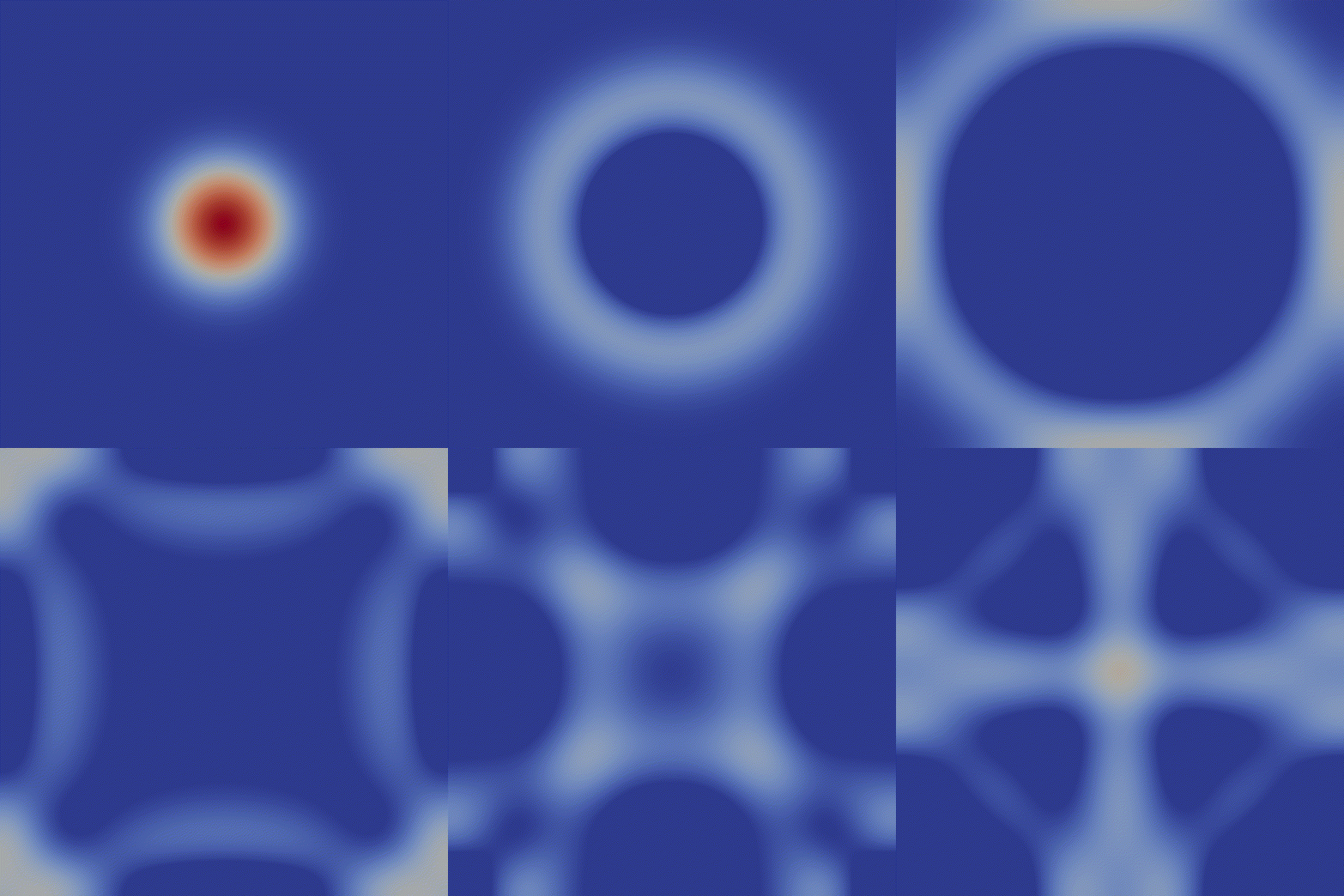
eta) for the full duration (1 second) of the problem.
Note
To run this example, you must first install SELF . We assume that SELF is installed in path referenced by the SELF_ROOT environment variable.
To run this example, simply execute
This will run the simulation from \(t=0\) to \(t=1.0\) and write model output at intervals of \(Δ t_{io} = 0.05\).
During the simulation, tecplot (solution.*.tec) files are generated which can easily be visualized with paraview.
